|
Algebra 2 will build on the topics of zeros, multiplicity, end behavior, and transformations as they relate to graphing. If you need to review your graphing skills,
see the "refresh" listings under Function Graphs.
|
A polynomial function is a function of the form
P (x) = anxn + an-1xn-1 + , , , + a2a2 + a1x + a0 ,
|
where the coefficients are real numbers
and the exponents are
non-negative integers. |
|
"P(x)" is often used to denote a polynomial function, but using "f (x)" is also appropriate.
NOTE: Keep in mind that not all polynomial functions have zeros (roots) that are Real Numbers.
Remember those quadratic graphs that float completely above the x-axis (never crossing or touching the x-axis),
because their polynomial roots
are complex numbers which do not lie on the x-axis.
The following discussion will deal with zeros (roots) that are Real Numbers.
Zeros or Roots:
 |
The "roots" of a polynomial are the |
| values of the variable (usually x), that make the polynomial's value equal to zero. |
|
In Algebra 1, you learned that the fastest way to find roots (or zeros), is to factor the polynomial, and then set the factors equal to zero. This process utilizes the zero factor principle which states that "if a • b = 0, then either a = 0 and/or b = 0."
Mathematically speaking, this connection between the factors of a polynomial and the zeros of the polynomial is stated as the Factor Theorem.
|
Factor Theorem: If f (x) is a |
| polynomial of degree n greater than or equal to 1, and "a" is any real number, then (x - a) is a factor of f (x) if and only if f (a) = 0. |
|
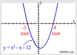
 The real numbers that create the "roots" of a polynomial correspond to the x-intercepts of the graph of the corresponding polynomial function, where the roots are referred to as "zeros". The real numbers that create the "roots" of a polynomial correspond to the x-intercepts of the graph of the corresponding polynomial function, where the roots are referred to as "zeros". |
The terms "root" and "zero" are often used interchangeably.
| Remember: A polynomial of degree 2 will have two roots (zeros), a polynomial of degree 3 will have three roots (zeros), and so on. |
|
Example:
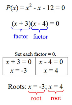
The values of -3 and 4
will now be referred to as
the zeros of the function.
|

What happens when a factor repeats?
Multiplicity of Zeros (or Roots):
In some situations, a polynomial graph will "cross" the x-axis at zero values. In other situations, the graph may simply "touch" (be tangent to) the x-axis at these points.
It is possible to determine whether a polynomial graph will "cross" the x-axis at each zero, or simply "touch" (be tangent to) the x-axis at each zero, before actually drawing the graph.
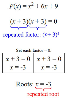
The example at the right is a simple polynomial of degree two (a quadratic), so there will be two zeros (roots). The factor of (x + 3) is repeated twice, and can also be written as (x + 3)2.
|
The number of times a factor appears in a polynomial is referred to as its multiplicity. |
|
In this example, (x + 3) has a multiplicity of 2, since it appears twice.
EVEN Multiplicity: When the multiplicity (the number of times a factor repeats) is an even number, the graph will just "touch" (be tangent to) the x-axis at that point. |
|
Example degree 2:
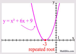 "just touching" or "tangent to"
the x-axis may also be referred
to as
"bouncing off" the x-axis.
|
What if the multiplicity is ODD?
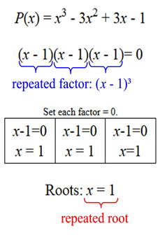
Consider the example at the right. The polynomial is of degree three, so there will be three roots (zeros). The factor of (x - 1) appears three times, and can be written as (x - 1)3.
Multiplicity ODD: When the multiplicity (the number of times a factor repeats) is an odd number, the graph will "cross" the x-axis at that point. |
Remember:
If you see a factor such as (x - 1)3, the multiplicity is 3.
If you see a factor such as (x + 2)2, the multiplicity is 2.
If you see a factor such as (x + 3), the multiplicity is 1.
Note: When you factor a polynomial, the sum of the multiplicities equals the degree of the polynomial.
x3 + x2 - 5x + 3 = (x - 1)2(x + 3) = (x - 1)2(x + 3)1
degree = 3
sum of multiplicities = 2 + 1 = 3 |
|
Example degree 3:
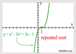 There is only one zero (root)
for this graph.
There is only one zero (root)
for this graph. |
Why do multiplicities work this way?
"EVEN" multiplicities mean the exponent of the factor is an even number. So, no matter what x-value is placed in "(x + 3)n, where n is even, the result will be positive. This means that this factor (being positive) will not change the "sign" of the function's expression, no matter what value is used for x in that factor. If the function was positive to the left of x = -3, it will remain positive to the right of x = -3, and the graph will just touch the x-axis, but not cross it.
In order for the function to cross the x-axis, the factor must be able to change the "sign" associated with the function's entire expression.
"ODD" multiplicities, using an odd power, will allow for the sign of the entire expression to be changed, and the graph to cross the x-axis, at which time the function's expression changes from positive to negative y-values (or vice versa).
Think of it this way:
In the function f (x) at the right, no matter what value of x is entered into the factor (x + 4)2, the sign of f (x) will never change. Multiplying by a positive value will not change the "sign" of the entire expression.
On the other hand, the factor (x - 1)3 has the power to change the sign of the expression since it can yield a potential negative result. Multiplying by a negative value can change an entire expression from + to -, or from - to +. |
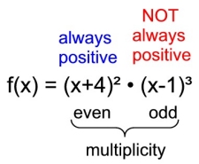
The sign "inside" the binomial
(x + 4) or (x - 1) does not matter. |
|
 Multiplicity is the number of times a factor appears in a polynomial. Multiplicity is the number of times a factor appears in a polynomial.
Multiplicity EVEN = graph is tangent to (just touches) the x-axis.
Multiplicity ODD = graph crosses x-axis. |
|
For
calculator help with finding
zeros.
click here. |
|
|
|
|

NOTE: The re-posting of materials (in part or whole) from this site to the Internet
is copyright violation
and is not considered "fair use" for educators. Please read the "Terms of Use". |
|
|