Binomial Probability and the Normal Curve MathBitsNotebook.com Topical Outline | Algebra 2 Outline | MathBits' Teacher Resources Terms of Use   Contact Person: Donna Roberts

Consider these questions:

Let's get some background information:

The super-imposed curve represents a normal distribution curve approximation for this binomial distribution.  You can see that it is a good fit.  The situation is such that as the number of tosses increases, the better the fit to the normal curve.  

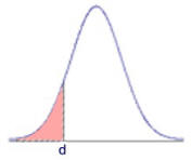
A normal distribution is really a continuous probability distribution.  On the normal distribution curve, the probability that an outcome is greater than d equals the area under the normal curve bounded by d and positive infinity.  The probability that an outcome is less than d equals the area under the normal curve bounded by d and negative infinity (as shaded in the diagram at the right).

Binomial distributions where p = 0.5 (such as this coin flipping example) are symmetric. When p is not equal to 0.5, the binomial distribution will not be symmetric.  The closer p is to 0.5 and the larger the number of trials, n, the more symmetric the distribution becomes.

In a binomial distribution with n trials and a success probability of p: The mean (expected value) is np. The variance is  . The standard deviation (standard error) is .

When the number of expected successes and failures is sufficiently large, an area under the normal curve will be a good numerical approximation of the exact binomial computation. RULE:  If np > 5 and n(1 - p) > 5, the normal curve will be a good approximation for the binomial distribution (usually good to two or three decimal places).

So how do we get the actual answer?

Binomial distributions deal with discrete variables which are made of whole units with no values between them, such as coin flips that are heads or tails, basketball tosses that make the hoop or not, or machine parts that are defective or not.  Normal distributions, however, deal with continuous variables which are endless in the number of times you can divide their intervals, such as gross pay, heights, or cholesterol levels.  To ensure the best approximation when dealing with these two variable types, we use a continuity correction factor.

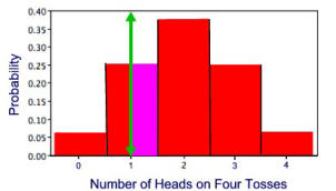
Continuity correction: Add or subtract 0.5 to the desired outcome to include the entire rectangle in the calculations. In the diagram at the right, if x is a binomial random variable, n = 4, p = 0.5, and we wish to compute the probability of x < 1 using the normal curve, we will miss the pink area. Adjustment:

Solving Question 2 using a normal approximation:  
Find the probability of getting at most 52 heads when flipping a fair coin 100 times.

Solution:  The facts:  n = 100, p = 0.5, q = 1 - p = 0.5, P(x < 52) = ?

1.  Check to see if "n" is large enough to warrant using a normal approximation.
Yes, n is large enough for the normal approximation to be accurate, since np = 50 > 5
(same for nq).

2.  Find the binomial standard deviation.
Use the formula:  .  The standard deviation for this problem is 5.

3.  Standardize the values of x using the Z-score formula:   . 
Remember to use x = 52.5 for the continuity correction.)

4.  See the Z-score chart to find the final answer:
Answer:  P(x < 52) = 0.6915

When dealing with very large samples, it can become very tedious to compute certain probabilities.  In such cases, the normal distribution can be used to approximate the probabilities that otherwise would have been obtained through laborious computations.

For working with At Most At Least on your calculator, click here.