When using sample statistics to make estimates of the values of population parameters, some statistics are much better at targeting these values and consequently yield better results. Statistics that are better at targeting population parameters are mean, proportion, variance and to a lesser degree standard deviation. We will be concentrating on the first two of these statistics.

Confidence Intervals and Levels:

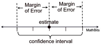
Once we have created our sampling distribution of the sample statistic, and arrived at our best estimate of the parameter of the population, we need to reveal just how good this estimate may be. Instead of simply stating the estimate as a single value, statisticians form intervals surrounding the estimate. These intervals are called confidence intervals (or interval estimates).

A confidence interval is a range, or interval, of values used to estimate the true value of a population parameter.

Confidence intervals are associated with confidence levels, such as 95%, which tell us the percentage of times the confidence interval actually contains the true population parameter we seek. The distance from the estimate to one end of a confidence interval is referred to as the margin of error (MOE). If you want to make a confidence interval smaller, increase the sample size.

Note: Correct statement: "We are 95% confident that the interval from 0.468 to 0.579 actually contains the true value of the population proportion." Incorrect statement: "There is a 95% chance that the true value of the population proportion lies between 0.468 and 0.579." The first refers to a 95% success rate of the process used. The second refers to the proportion itself.

Dealing with Proportions • For ALL possible samples of the same size, n, from the same population, the graph of the sampling distribution of sample proportions will resemble a Normal curve with a mean equal to the value of the true population proportion.

Notations: population mean = μ (mu) population proportion = p population standard deviation = σ sample mean = (x-bar) sample proportion = (p-hat) sample standard deviation = s

• Standard error (SE) is the standard deviation of the sampling distribution of a statistic (for proportions, ).

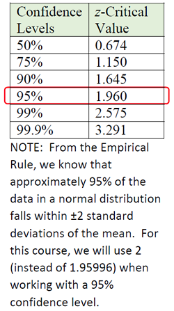
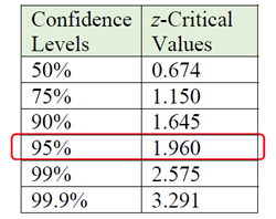
• To obtain the margin of error (MOE) for working with a sample proportion, we need to address the Confidence Level needed in the problem (such as 95%). To do this, multiply the standard error by the critical value associated with the desired Confidence Level (see chart at the right and read the NOTE). For a confidence level of 95%, we use the formula: Since we are familiar with 95% being associated with ±2 standard deviations of the mean, we will be using 2 for the Critical Value associated with a 95% Confidence Level. If you are using the other Confidence Levels, use the values from the chart (instead of 2) in the formula.

When data from a simple random sample are used to estimate a population proportion, p, the margin of error, MOE, is the maximum expected difference between the observed sample proportion,, and the true value of the population proportion, p. • Example: If the sampling mean proportion is 0.32, the sample size is 40, and we want a confidence level of 95%, the formula tells us that the MOE is 0.148. We are 95% confident that the interval 0.32 ± 0.148 includes plausible values for the true proportion.  (0.172 < p < 0.468)

Dealing with Means (where population standard deviation is known)

• In this situation, we know the population standard deviation and we seek the population mean, μ. This is an unlikely scenario, since if we know ALL of the population to get σ, we would know μ. But it does offer the opportunity for some statistical investigation.

• For ALL possible samples of the same size, n, from the same population, the graph of the sampling distribution of the sample means will resemble a Normal curve with a mean equal to the value of the true population mean.

• The differences between μ andtend to be smaller than the differences obtained with some other statistics, such as the median. Sample means tend to target the value of the population mean.

• To obtain the margin of error (MOE) for working with sample means, we need to address the confidence level needed in the problem (such as 95%). To do this, multiply the standard error by the critical value associated with the desired confidence level (see chart at the right. Remember that we will be using 2 (not 1.96) for the 95% confidence level.). For a confidence level of 95%, we use the formula:

Remember: As seen in the section above "Dealing with Proportions", we are using a Critical Value of 2 for a Confidence Level of 95% instead of a Critical Value of 1.960.

For a 95% Confidence Level, we are using 2 (instead of 1.960). If you are using the other Confidence Levels, use the values from the chart (instead of 2) in the formula.

• Example: If the population standard deviation is known to be 0.675, sample mean is 72.5, sample size is 40, and we want a confidence level of 95%, the formula tells us that the MOE is 0.213. We are 95% confident that the interval 72.5 ± 0.213 includes plausible values for the true mean.   (72.29 < μ < 72.71)

Given the standard deviation (SE) of the sampling distribution of the sample mean (), the MOE formula for a 95% Confidence Level is simply 2•(standard deviation).

** We will not be "Dealing with Means where population standard deviation is NOT known" in this course. For our purposes, should we not be given the population standard deviation, we will use our best estimate, which will be the sample standard deviation. The degree of uncertainty this creates, however, will require an adjustment from z-Critical Values to t-Critical Values which is left for another course.

Side-Notes:

• While increasing the sample size does not have a profound effect on the mean, it does have an effect on the standard deviation. Thus, a larger sample size will create a smaller margin of error, due to the decrease in the standard deviation.

• The smaller the standard error, the higher the precision of the statistic for estimating a population parameter.

• In dealing with margin of error (MOE), some authors will refer to the use of 2, instead of 1.960, regarding 95% confidence levels, as an "Approximate MOE" while the use of 1.960 is the "Exact MOE". Most will agree, however, that it rarely makes a difference in the calculations.

• It is known that standard deviation is a measure of how far values in a population tend to be from the population mean.  It measures the spread of the values in the population.  When working with sampling distributions, the standard error is the standard deviation with a slightly different interpretation. The standard deviation of a sampling distribution is a measure of how far a sample mean or sample proportion tends to be from the true population mean or population proportion.

• When working with sampling distributions, the sample size should be sufficiently large as to ensure that the samples are independent. The sample size must be large enough to make the sampling distribution model approximately Normal. The sample size should not exceed 10% of the population. Samples are almost always drawn without replacement. If the sample exceeds 10% of the population, the probability of a success changes so much during sampling that a Normal model may no longer be appropriate. In addition, the sample size should be large enough to expect at least 10 "successes" and at least 10 "failures" in the sample data.

Example:

Let's investigate the following statement:

If all possible samples of a certain size, n, are selected from a population, the mean of these sample means will be equal to the population mean.

We will be using a small population to make the formation of the sample sets easier.

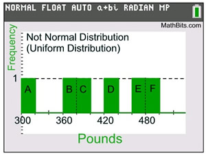
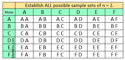
Population: The weight of 6 mini-mules in pounds. Population Data: {300, 360, 380, 420, 460, 490} Population Size: N = 6 Population Mean: 401.6666667pounds Population Standard Deviation: 63.35525936 pounds Population Graph: Uniform Distribution Let's find ALL possible samples of size n = 2 for this population.

	There will be a total of 36 possible sample sets of size n = 2 from this population.
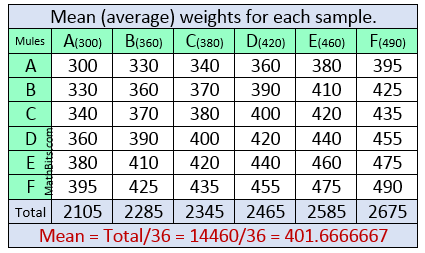
	Find the mean of each sample set. This list of 36 "means" creates the Sampling Distribution of Sample Means. Find the mean (average) of the means of all of the sample sets. This is the mean of the Sampling Distribution. Notice that the mean of the Sampling Distribution is exactly the same as the population mean (401.6666667).
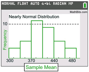
	The graph of the Sampling Distribution of the Sample Means is nearly a Normal Distribution. Remember that the graph of the population was a Uniform Distribution graph. The graph of the sampling distribution of a sample statistic is always Normal, or nearly Normal.
Sample Size: n = 2 Sampling Distribution of Sample Means Mean: 401.6666667pounds Sampling Distribution of Sample Means Standard Error: 44.79893352 pounds Sampling Distribution of Sample Means Graph: Nearly Normal Distribution Notice that the standard deviation (SE) of the Sampling Distribution of Sample Means is smaller than that of the population.