We have seen the use of linear, quadratic, exponential, and power regressions. On this page we will investigate how logarithmic and sinusoidal equations can be used as regression models.
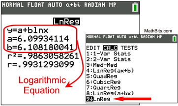
Logarithmic Regression (LnReg) |
|
 Characteristics:
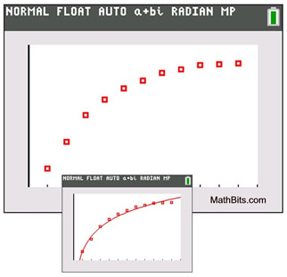
• The scatter plot appears to resemble the shape of the function y = ln( x).
• Form: y = a + b ln( x)
• The calculator takes the natural log of the x-coordinates and then preforms a linear regression. Thus any x-coordinate that is negative or zero will cause an ERR DOMAIN on the calculator.
|
|
• The logarithmic regression equation will be used to predict y-values that lie inside (interpolate) or outside the plotted values (extrapolate).
• Like the exponential function, the logarithmic function can be transformed to be a linear based regression.
Logarithmic regressions are widely used to model environmental data.

|
Sinusoidal Regression (SinReg) |
 The mathematical sinusoidal function and
the calculator's sinusoidal regression equation are slightly different.
Mathematical
Sinusoidal Function
y = Asin(B(x - C) + D
| A | = amplitude
B = frequency
period = 2π / B
D = vertical shift
C = horizontal shift
(called phase shift when B = 1) |
Calculator's
Sinusoidal Regression Equation
y = asin(bx + c) + d
| a | = amplitude
b = frequency
period = 2π / B
d = vertical shift
c / b is the horizontal shift
(right if c < 0 and left if c > 0)
|
|
|
 Characteristics:
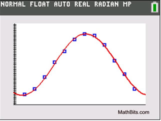
• The scatter plot appears to resemble a sine or cosine curve.
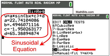
• Form: y = a sin(bx+c) + d
|
| • Notice that there is no correlation coefficient, r, or coefficient of determination, r2, listed for this regression. |

